Chaining Reactive Functions
Contents
Chaining Reactive Functions
One of the reasons reactive functions are so powerful is that they can be chained together. This allows us to decompose code into neatly abstracted functions and then compose them together to create complex workflows.
Let’s look at an example with two reactive functions, add and multiply.
@mk.reactive()
def add(a, b):
    return a + b


@mk.reactive()
def multiply(a, b):
    return a * b


x = mk.Store(1)
y = mk.Store(2)

u = add(x, y)  # u is Store(3), type(u) is Store
v = add(y, 7)  # v is Store(9), type(v) is Store
w = multiply(u, 2)  # w is Store(6), type(w) is Store

x.set(4, triggers=True)
# u is now Store(6), type(u) is Store
# v is unchanged
# w is now Store(12), type(w) is Store
Let’s break down this example:
addandmultiplyare both reactive functions.udepends onxandy, so it will be updated if either of them are updated.vdepends only ony, so it will only be updated ifyupdates.wdepends onu, so it will be updated ifuis updated.
When we update x, only u and w are updated, by running add and multiply again respectively. If instead we updated y, all three outputs u, v and w would be updated, with add running twice and multiply running once.
In practice, Meerkat provides in-built reactive functions for many common operations on Store objects. So we could have written the example above as:
x = mk.Store(1)
y = mk.Store(2)

u = x + y  # u is Store(3), type(u) is Store
v = y + 7  # v is Store(9), type(v) is Store
w = u * 2  # w is Store(6), type(w) is Store
In the above example, the + and * operators were automatically turned into reactive functions. Other examples include mk.len(), mk.str(), and mk.sort(). You can find a full list of the reactive functions that Meerkat provides here.
One place where chaining can be helpful is when you want to create a function that takes a DataFrame as input, and returns another DataFrame as output (a “view” of the original DataFrame). Let’s look at an example.
@mk.reactive()
def filter(df, column, value):
    return df[df[column] == value]

@mk.reactive()
def sort(df, column):
    return df.sort(column)

@mk.reactive()
def select(df, columns):
    return df[columns]

df = mk.DataFrame({
    "a": [random.randint(1, 10) for _ in range(100)],
    "b": [random.randint(1, 10) for _ in range(100)],
})
filtered_df = filter(df, "a", 2)
sorted_df = sort(filtered_df, "b")
selected_df = select(sorted_df, ["b"])
Here, we filter, sort and select columns from a mk.DataFrame, chaining these reactive functions together to achieve this effect. Again, in practice, Meerkat provides reactive functions for many common operations on mk.DataFrame, so we could have written the example above as:
filtered_df = df[df["a"] == 2]
sorted_df = filtered_df.sort("b")
selected_df = sorted_df[["b"]]
This pattern works with
mk.DataFrameand notpandas.DataFrame. If you’re using apd.DataFrame, we recommend converting to amk.DataFrameusingmk.DataFrame.from_pandas(df)when using Meerkat’s interactive features.Alternately, you can also use the
magiccontext manager if you want to “turn on” the same functionality forpd.DataFrameobjects. We recommend reading the guide at XXXXXXX to learn more about this.
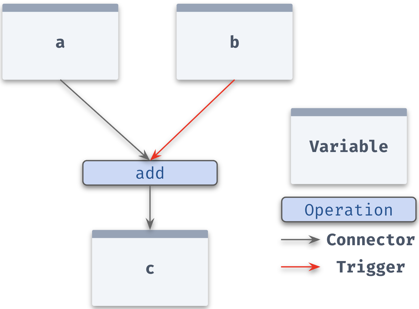
Reactivity as a Graph
We can think of reactivity as a graph of inputs, functions, and outputs. In fact, Meerkat maintains a graph of reactive functions and their inputs and outputs to determine what functions should be rerun.
What are the nodes?
Reactive functions and their inputs and outputs are all nodes in the graph.
When a reactive function is called with inputs, a node is created for the function call and its inputs.
The node for the function call is referred to as an Operation.
The operation corresponds to this particular function call. If the function is called again, a new operation is created.
What are edges in this graph? Edges indicate what variables are inputs to a function, and what variables are outputs of a function. These edges are directed - i.e. input -> operation -> output.
There are two kinds of edges in the graph:
Trigger Edges: These edges indicate which variables should trigger an operation to rerun.
Connector Edges: These edges simply indicate that variables are inputs/outputs (i.e. connected) to an operation. Connector edges between an input and an operation indicate that changes in the input will not trigger the operation to rerun.
Trigger edges are used to describe relationships between inputs and the operation. In other words, an input triggers an operation to rerun if the input points to the operation with a trigger edge.
This distinction is important because it allows us to be selective about which inputs should trigger a function to rerun.
For example, c = add(a,b) only reruns when b changes.
@mk.reactive()
def add(a, b):
    return a + b

a = mk.Store(1).unmark()
b = mk.Store(2)
c = add(a, b)
The graph looks like this: